1. Introduction
For two decades the literature on card fraud detection has accumulated reported architecture gains that rarely survive methodological scrutiny — the phenomenon Hand (2006) named the illusion of progress. Hayat and Magnier (2025) documented this dynamic specifically on the ULB/Worldline benchmark: preprocessing leakage, inadequate temporal validation and selective metric reporting jointly produce trivial neural networks with an apparent recall of 99.9%. This paper addresses a complementary question: even under a correct protocol, how much of the reported operational performance is due to the chosen architecture — and how much is due to a single scalar, the decision threshold?
The question matters because the two levers carry radically different engineering costs. Switching model family costs retraining, revalidation and a new sign-off; shifting the operating point costs the choice of one number on validation, is auditable line by line and is reversible. If the effect of the latter dominates the effect of the former, the effort priority of fraud engineering — and the proper object of model governance — has been historically inverted. Multi-domain evidence in this direction already exists: across 9,000 experiments over 30 datasets, decision-threshold calibration was the most consistently effective intervention against imbalance, ahead of SMOTE and of class reweighting (Abdelhamid & Desai, 2024). The delta of this work is deliberately modest: to give that decomposition — already indicated, without paired inference, by Leevy et al. (2023) and by Abdelhamid and Desai (2024) — paired intervals, a training-variance yardstick and an auditable protocol, on the canonical benchmark of the fraud literature, whose citing community around Hayat and Magnier (2025) still does not adopt the practices it cites.
This is, deliberately, a confirmatory and auditable case study — not the proposition of a new thesis. The contributions are three, plus a note. First, the decomposition: with a paired bootstrap of 10,000 replicates and a training-variance study over 20 seeds, it is shown that shifting the threshold moves the MLP test F1 by +0.545 (from 0.267 to 0.812), whereas the gap between MLP and Logistic Regression under the correct selection regime is −0.007 [−0.055, +0.042] — indistinguishable from zero, smaller than the training standard deviation of the MLP itself (0.016) and with a sign that flips in 12 of the 20 seeds. Second, the reproducible operationalization of the critique: standardization fitted on the training split alone, cost reweighting in place of any synthetic oversampling, threshold selected exclusively on validation, SHA-256-anchored data, protocol invariants covered by automated tests and determinism verified by bit-identical re-execution. Third, a reproducibility forensic of the author's own precedent material, from which two findings result: the apparent superiority of the MLP produced by censoring the threshold grid (Section 6.2) and a resampling defect that invalidated the prevalence-robustness test (Section 6.5). The regulatory implications of the thesis — including the correction of a current reading of Regulation (EU) 2024/1689 — are treated in the Discussion (Section 7).
The central trade-off of the problem has a classical name: it is the Neyman-Pearson decision boundary in precision-recall space, under a cost asymmetry in which false negatives (undetected fraud) cost orders of magnitude more than false positives (a legitimate transaction blocked) (Bishop, 2006; Cherif et al., 2023; Fawcett, 2006).
2. Related work
Three lineages converge in this study. The first is that of methodological critique. Hand (2006) argued that marginal gains from sophisticated classifiers rarely survive outside the laboratory; Kapoor and Narayanan (2023) systematized the taxonomy of data leakage as the engine of the reproducibility crisis in machine-learning-based science; Boulesteix and Strobl (2009) quantified the optimistic bias induced by model selection on the evaluation set itself. In the card fraud niche, Kabane (2024) demonstrated that resampling applied before the split inflates XGBoost metrics on the same ULB dataset, and Hayat and Magnier (2025) consolidated four systemic failures of the benchmark literature. The community response to that critique has so far been to cite it and ignore it: the works that reference it keep reporting state of the art on the same benchmark without changing protocol.
The second lineage is that of the operating point and of cost. The optimal threshold for F1 and its relation to calibrated probabilities were formalized by Lipton et al. (2014); King and Zeng (2001) had already shown that logistic models underestimate rare events without correction. Contemporary evidence is convergent (for a panorama of the field, Chen et al., 2024): imbalance corrections by resampling degrade calibration without discriminative gain (van den Goorbergh et al., 2022); synthetic oversampling does not benefit strong classifiers, and adjusting the operating point suffices (Elor & Averbuch-Elor, 2022); threshold calibration is the most consistent intervention across 15 models and 30 datasets (Abdelhamid & Desai, 2024); and synthetic fraud samples generated by CTGAN degraded both individual models and fusions on the IEEE-CIS benchmark (Han & Wu, 2026). On the ULB dataset itself, Leevy et al. (2023) compared threshold optimization with and without random undersampling — obtaining the best results without the undersampling —, and Ngoc Thanh Sang (2026) proposed exactly the recipe adopted here — cost-weighted loss, threshold calibration and leakage-aware validation. None of these works, however, decomposes and compares the threshold effect against the architecture effect with paired inference, nor publishes the protocol with tests, hashes and determinism verification; that is the gap this case study fills. The institutionalization of the practice confirms its maturity: since 2024 the scikit-learn 1.5 library (Pedregosa et al., 2011) exposes post-training threshold tuning as a first-class API, TunedThresholdClassifierCV.
The third lineage explains why the tie between architectures was expectable a priori. Grinsztajn et al. (2022) identified that neural networks are approximately rotation-invariant, whereas trees exploit the axis alignment of the original variables — and the V1–V28 variables of the ULB dataset are principal components (PCA), that is, the result of a rotation. If the PCA projection makes the classes approximately separable by a linear boundary, linear models and MLPs saturate the same signal ceiling (Hastie et al., 2009). McElfresh et al. (2023) add, over 176 tabular datasets, that light hyperparameter tuning on boosted trees frequently matters more than the choice between neural networks and trees itself. Finally, the training instability of deep networks is documented by Bouthillier et al. (2021): routinely ignored sources of variance — data sampling, weight initialization, hyperparameter choice — markedly impact results and distort the detection of improvements between methods; this study measures that variance directly in the case at hand (Section 6.3).
3. Data
The ULB/Worldline dataset, maintained by the Machine Learning Group of the Université Libre de Bruxelles and distributed via Kaggle, contains 284,807 transactions from two days of September 2013, with 30 predictor variables — 28 anonymized principal components (V1–V28), the elapsed time (Time) and the amount (Amount) — and a binary label Class with 492 frauds (prevalence of 0.173%; Figure 1) (Dal Pozzolo, 2015; ULB/Worldline, 2013). The copy used was verified against the SHA-256 recorded in the original execution of the precedent material (76274b691b16a6c49d3f159c883398e03ccd6d1ee12d9d8ee38f4b4b98551a89), ensuring bit-for-bit identity of the data chain between the two executions.
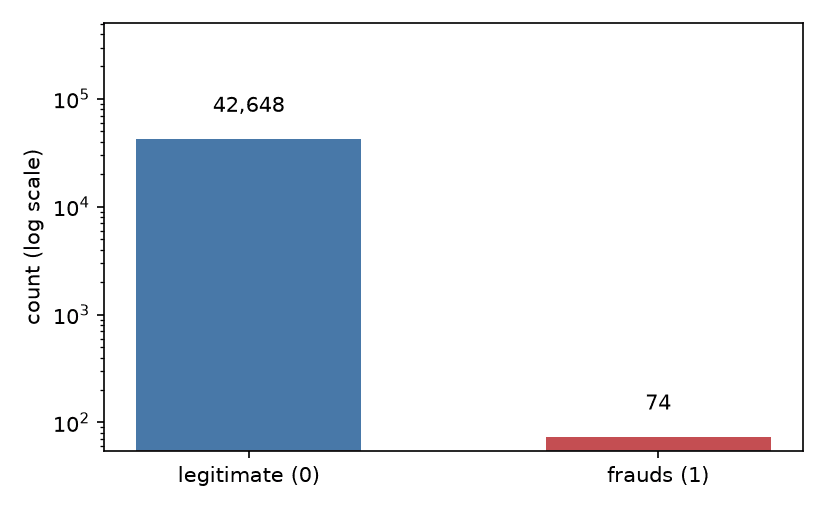
The scientific role assigned to the benchmark here is deliberately restricted. As a leaderboard, the dataset is saturated and compromised: metrics above 99% are a symptom of leakage, not of progress (Hayat & Magnier, 2025; Kabane, 2024); PCA anonymization may, in the limit, preserve 99.9999% of the variance and still destroy the decision signal (Tembine, 2026); and modern curated tabular suites exclude it because of the extreme imbalance. As a methodological instrument for decomposing protocol effects — the use made in this paper — it remains adequate, precisely because it is the benchmark on which the biased conclusions of the literature were built.
4. Methods
Provenance note: this paper reanalyzes unpublished precedent material by the author himself (technical report and computational notebook of August 2025; Flores, 2025). Reconciling the text of that report with the code actually executed revealed material divergences — the text described SMOTE oversampling and probability calibration (Platt and temperature scaling) that the code never executed, besides an architecture different from the one implemented. This paper describes and reports exclusively what the code executes; the original notebook, with its SHA-256 hash recorded, accompanies the replication package (Flores, 2026) as archival material.
The protocol, entirely configured by file and covered by invariant tests, is the following. The split is stratified 70/15/15 (training/validation/test) with seed 42, yielding 199,364/42,721/42,722 transactions and 344/74/74 frauds, respectively. Standardization (StandardScaler) is fitted exclusively on the training split and applied to the remaining ones — the class of preprocessing leakage denounced by Hayat and Magnier (2025) and Kabane (2024) is therefore excluded by construction. No synthetic oversampling — SMOTE (Chawla et al., 2002) or derivatives — is used: the imbalance is handled by cost reweighting, with the positive-class weight equal to the ratio between negatives and positives in the training split (199,020/344 ≈ 578.5) in the MLP loss function and class_weight="balanced" in the Logistic Regression — a choice aligned with the evidence that resampling distorts the posterior probability and degrades calibration without discriminative gain (Dal Pozzolo et al., 2015; Elor & Averbuch-Elor, 2022; van den Goorbergh et al., 2022).
Four families are compared. The MLP (PyTorch 2.6.0) has a 30-64-32-1 architecture with BatchNorm, ReLU and Dropout of 0.2 per hidden layer, Adam optimizer (rate 10⁻³), binary cross-entropy loss with the pos_weight above, 40 epochs, batches of 512 and selection of the best state by validation F1 at threshold 0.5 (Goodfellow et al., 2016). The Logistic Regression (LR) uses the liblinear solver with up to 200 iterations (King & Zeng, 2001). The Autoencoder (30-64-32-8, mirrored) trains for 40 epochs on legitimate training transactions only and scores by the squared reconstruction error (Pang et al., 2021). The Isolation Forest uses 200 trees, automatic contamination and training on legitimate transactions only (Liu et al., 2008). No model receives probability calibration; scores are treated as ordinal and the threshold as an operating point on the score scale — not as a probability. Under cost reweighting with a factor of ~578, the scale compresses towards 1, and the default threshold of 0.5 (de facto the libraries' default) ceases to correspond to any reasonable operating point — a fact central to the results.
Threshold selection occurs exclusively on validation, in two regimes reported separately. The fidelity regime reproduces the grid of the precedent material, 99 uniform points in [0.01, 0.99] — a right-censored grid, since the optimum may lie beyond 0.99. The primary regime removes the censoring, evaluating every cutoff point of the validation precision-recall curve. For the Autoencoder and the Isolation Forest, the cutoff is selected over percentiles (50 to 99.9) of the validation score, as in the precedent material. Inference on the gap between MLP and Logistic Regression uses a paired bootstrap of 10,000 replicates over the test indices, reporting 95% percentile intervals for the F1 of each model, for the paired F1 difference and for the paired AUC-PR difference; these intervals capture the sampling variance of the test set conditional on the trained models and fixed thresholds — not the training variance, measured separately by 20 MLP retrainings with seeds 1–20 over a fixed split and standardization. Execution is deterministic (fixed seeds, single thread, deterministic algorithms): two complete executions produced identical results in every block, and all artifacts — code, configuration, results, tables and figures — are recorded in a manifest with individual SHA-256.
5. Evaluation protocol
The primary metric is the area under the precision-recall curve (AUC-PR), more informative than the ROC under severe imbalance because it ignores the abundant true negatives (Davis & Goadrich, 2006; Saito & Rehmsmeier, 2015); the ROC is reported by tradition (Fawcett, 2006). Pointwise performance uses F1 and Fβ with β=2 at the threshold selected on validation — weighting recall over precision reflects the asymmetric cost of the domain, a recurrent practice in the fraud literature (Hernandez Aros et al., 2024) —, complete confusion matrices and accuracy only as an illustration of its uselessness in the rare-class regime (99.2% at threshold 0.5 coexisting with a precision of 0.157). Interpretability uses permutation importance on validation (5 repetitions, with standard deviation). Prevalence sensitivity is treated analytically in Section 6.5.
6. Results
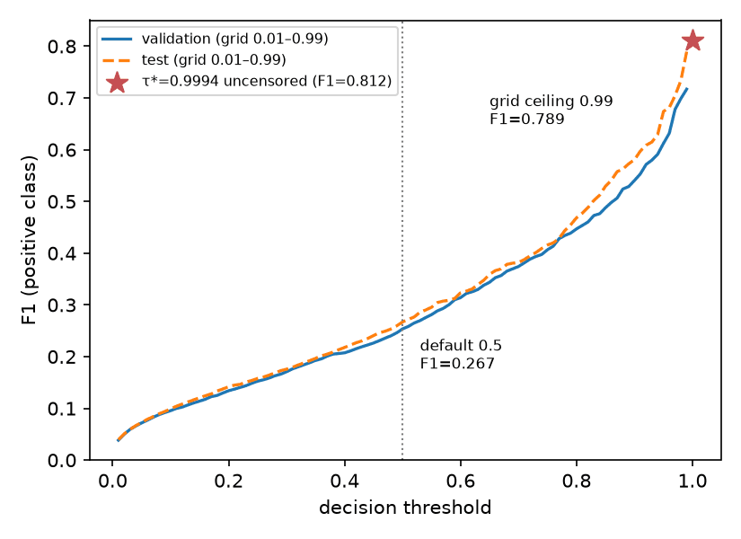
Table 1 consolidates performance by model and operating point on the test set; Figure 2 (precision-recall curves) and Figure 3 (threshold sweep) support the reading of Sections 6.1 and 6.2.
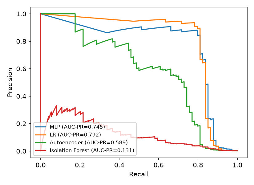
Table 1 — Test performance by model and operating point (source: results.json of the replication package).
| Model and threshold | Precision | Recall | F1 | FP | FN |
|---|---|---|---|---|---|
| MLP, 0.50 | 0.157 | 0.878 | 0.267 | 348 | 9 |
| MLP, 0.99 | 0.769 | 0.811 | 0.790 | 18 | 14 |
| MLP, τ* | 0.875 | 0.757 | 0.812 | 8 | 18 |
| LR, τ* | 0.931 | 0.730 | 0.818 | 4 | 20 |
| Autoencoder | 0.769 | 0.405 | 0.531 | 9 | 44 |
| Isolation Forest | 0.112 | 0.459 | 0.179 | 271 | 40 |
Note. Values rounded to three decimal places. 0.50 = library default threshold; 0.99 = ceiling of the censored grid (v3.2 fidelity); τ* = uncensored validation optimum (MLP 0.9994; LR ≈1.0); Autoencoder and Isolation Forest at the F1-optimal validation cutoff.
6.1. The effect of the operating point
Shifting the MLP threshold from 0.5 to the optimum selected on uncensored validation (τ* = 0.9994) moves test F1 from 0.267 to 0.812 — a gain of +0.545 obtained by a single scalar, without touching architecture, weights or data (Figure 3).
In operational terms, false positives fall from 348 to 8 (−97.7%) at the cost of 9 true positives (65→56); Figure 4 contrasts the confusion matrices at the two points.
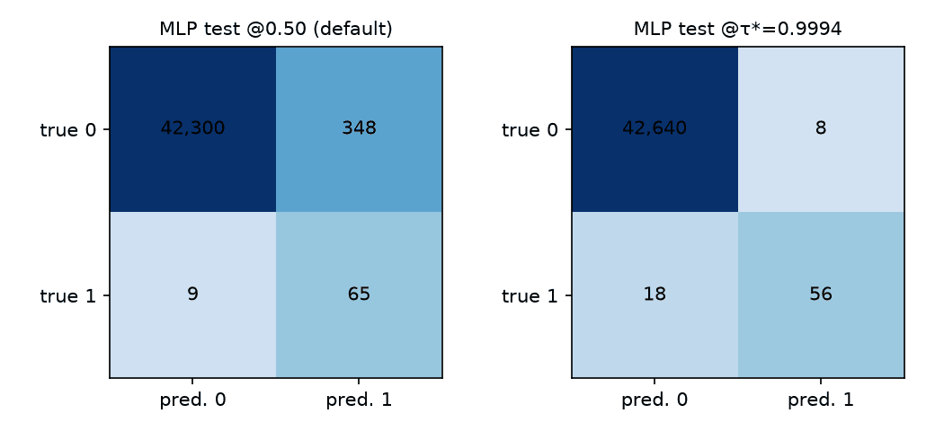
Fβ=2, which weights recall over precision, reaches 0.779 on the test set at the corresponding threshold. Comparing the threshold swing with the gap between architectures requires a commensurability caveat: the first corrects a misconfiguration (the 0.5 default is a catastrophic operating point under cost reweighting), whereas the second compares alternatives that are both optimized. That is exactly the engineering message: the cheap and auditable correction precedes — and exceeds in effect, here by two orders of magnitude — the expensive architecture decision.
6.2. The gap between architectures and the censoring artifact
Under the primary regime, MLP and Logistic Regression are statistically indistinguishable: F1 of 0.812 against 0.818 (ΔF1 = −0.007; paired 95% CI [−0.055, +0.042], containing zero with room to spare) and AUC-PR of 0.745 against 0.792 (ΔAUC-PR = −0.046; CI [−0.111, +0.005], containing zero). The fraction of bootstrap replicates favorable to the MLP is 38% in F1 and 4% in AUC-PR — opposite signs across metrics, a classic symptom of an ill-conditioned effect. The correct reading of the indistinguishability should be recorded: with 74 positives in the test set the interval is wide, and absence of evidence of difference is not evidence of equivalence — a real gap of up to ±0.05 in F1 is compatible with these data; what the data do sustain is that any gap of that order is smaller than the effect of the threshold and than the training variance itself (Section 6.3).
Table 2 confronts the two selection regimes; Figure 5 shows the bootstrap distribution of the paired difference under the primary regime.
![Histogram of the 10,000 paired bootstrap replicates of ΔF1 = F1(MLP) − F1(LR) on the test set, roughly symmetric and centered slightly left of zero, with dashed lines at the 95% interval [−0.055, +0.042] and the zero line well inside it.](/_next/image?url=%2Fresearch%2Foperating-point-dominance%2Ffig5-en.png&w=1920&q=75)
Table 2 — Paired bootstrap MLP × Logistic Regression on the test set (10,000 replicates, 95% percentile CI), by threshold-selection regime.
| Quantity | Censored grid (v3.2 fidelity) | Uncensored (primary) |
|---|---|---|
| τ* MLP / τ* LR (validation) | 0.99 / 0.99 (grid ceiling) | 0.9994 / ≈1.0 |
| F1 MLP (test) | 0.790 | 0.812 [0.735, 0.877] |
| F1 LR (test) | 0.736 | 0.818 [0.739, 0.884] |
| ΔF1 (MLP−LR) | +0.053 [+0.019, +0.093] | −0.007 [−0.055, +0.042] |
| ΔAUC-PR (MLP−LR) | −0.046 [−0.111, +0.005] | −0.046 [−0.111, +0.005] |
| Replicates favorable to the MLP (F1) | 99.9% | 38.5% |
The fidelity regime produces the opposite — and instructive — result. With the inherited grid censored at 0.99, the MLP appears to win with significance: ΔF1 = +0.053, CI [+0.019, +0.093], excluding zero. The cause is mechanical: under cost reweighting, scores compress towards 1 and the optima of both models lie beyond 0.99 (τ*MLP = 0.9994; τ*LR ≈ 1.0); the grid ceiling bites the two unequally, and the difference in scale compression — not discriminative capacity — decides the "winner". An arbitrary sweep limit, inherited without examination, manufactures an architecture conclusion with the appearance of statistical rigor. This is the central instructive result of the study — a failure mode predictable in hindsight, yet routinely inherited without examination, given that truncated grids such as [0.01, 0.99] are idiomatic in tutorials and reference code: neither classic leakage nor chance, but a protocol micro-decision, suffices to flip the qualitative conclusion of a model comparison.
6.3. Training variance: the gap within the model's own noise
Twenty MLP retrainings (seeds 1–20; split, standardization and protocol fixed; threshold again selected on validation per seed) produce test F1 with mean 0.814, standard deviation 0.016 and range 0.7879–0.8429. The Logistic Regression, deterministic, scores 0.8182 — within half a standard deviation of the MLP mean. The per-seed gap ranges from −0.030 to +0.025, and the MLP beats the LR in only 8 of the 20 seeds. Ceteris paribus, retraining the same model shifts the result more than replacing it with the linear baseline — a local quantification of the phenomenon that Bouthillier et al. (2021) documented at scale: ignored sources of variance exceed the deltas published between methods. The cross-platform observation should also be recorded (n=2, illustrative): the same configuration with seed 42 produced F1 of 0.747 in the original environment (Colab, x86, multi-thread) and 0.789 in the local deterministic re-execution (ARM, single thread) — a difference of 0.042, again larger than the gap between architectures.
6.4. Unsupervised detectors
Autoencoder and Isolation Forest fall substantially below the supervised models (F1 of 0.531 and 0.179 against ~0.81), confirming that, with labels available, supervised learning with reweighting dominates detection by structural deviation (Liu et al., 2008; Pang et al., 2021). The Autoencoder further exhibits qualitative instability between executions of the same protocol: in the original execution it reached F1 of 0.215 with 300 false positives (precision 0.130); in this one, 0.531 with 9 false positives (precision 0.769) — opposite failure modes, produced by the sensitivity of the percentile cutoff over the tail of the reconstruction error. An observation with n=2, reported as a practical warning: percentile thresholds over reconstruction scores are fragile by construction.
6.5. Prevalence sensitivity: forensics and closed form
The precedent material reported F1 stability under prevalence variation from 1% to 20%. Forensic analysis of the code revealed that the test never reached the nominal prevalences: the resampling used size=min(n_pos, 74), locking the positives at 74 and the effective prevalence between 0.17% and 0.22% in every scenario — the "stability" measured bootstrap replicates of the test set itself, not robustness to prior shift. The verification, reproducible in the replication package (Flores, 2026), replicates both variants over the same scores: the defective one produces a flat F1 (0.770–0.786); the corrected one reaches the nominal prevalences.
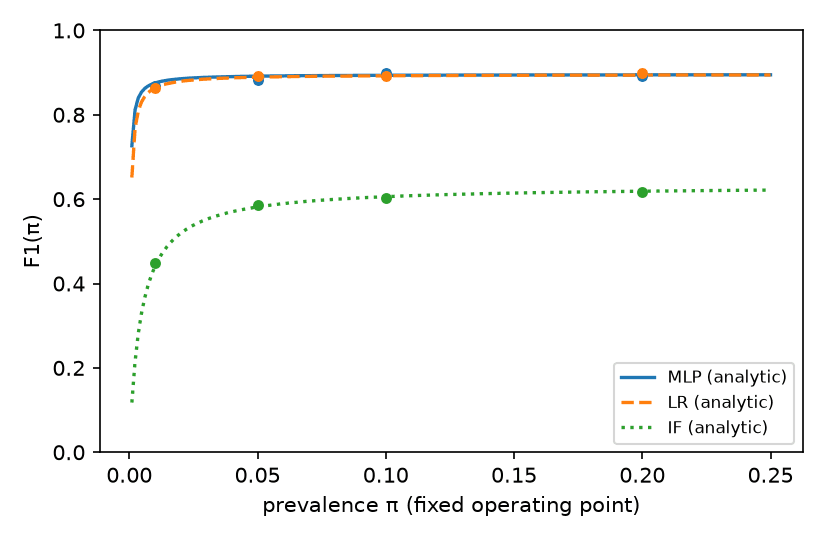
Once the defect is corrected, the correct sensitivity dispenses with simulation: with a fixed operating point, the true-positive (TPR) and false-positive (FPR) rates are invariant to prevalence π, and precision follows the identity prec(π) = π·TPR / (π·TPR + (1−π)·FPR), from which F1 derives in closed form (Figure 6, with pointwise Monte Carlo verification). This analysis deliberately uses the operating point of the fidelity grid (τ=0.99), the same one as the original test being corrected — not the primary regime of Section 6.2 —, so that the comparison with Table 3 of the precedent material is point by point. For the MLP at that cutoff (TPR 0.811; FPR 4.2×10⁻⁴), the analytical F1 grows from 0.875 at π=1% to 0.895 at π=20% — a mechanical growth of precision with prevalence, not an improvement of the model; for the Isolation Forest (FPR 15 times larger), from 0.440 to 0.619. The honest reading is twofold: the F1 metric is a function of prevalence even with a frozen detector, and therefore a threshold fixed for 0.17% changes operational meaning under another base rate — one further argument for treating the operating point, and not the architecture, as the live governance artifact (Dal Pozzolo et al., 2018).
6.6. Permutation importance
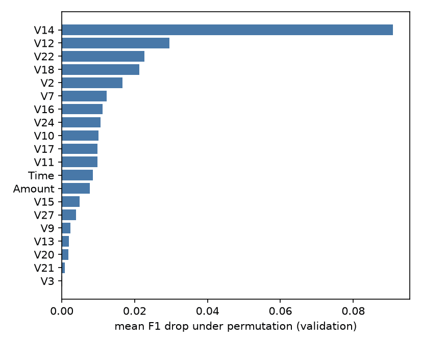
V14 dominates permutation importance on validation (0.091 ± 0.013; Figure 7), about three times the second variable (V12, 0.030 ± 0.008) — but the secondary ranking differs from the one obtained in the original execution (V2 in second place), reiterating the instability of fine conclusions under retraining. Two caveats preclude a causal reading: marginal permutation importance is biased in the presence of correlation (Strobl et al., 2008) — mitigated, but not eliminated, by the constructive orthogonality of the PCA components — and an anonymous principal component is not a fraud mechanism; the variance-preserving rotation may even destroy the relevant decision information (Tembine, 2026).
7. Discussion
The tie between MLP and Logistic Regression is not an accident of this dataset; it is the behavior predicted by the third lineage of Section 2. Neural networks hold no structural advantage over linear boundaries when the representation has already been rotated by PCA and the remaining signal is approximately linearly separable (Grinsztajn et al., 2022; Hastie et al., 2009); what the empirical comparison adds is the scale of the non-effect: smaller than the training variance of the MLP itself, with a sign that depends on metric, seed and a grid ceiling. A ranking with these properties does not constitute a rational basis for an architecture decision — whereas the shift of the operating point, two orders of magnitude larger, is measurable, cheap and auditable.
The deliberate absence of probability calibration delimits the reach of the conclusions. Threshold selection by F1 on validation is an operating-point decision over ordinal scores — valid as a ranking, and it is all this study requires. Converting the threshold into an expected-cost policy (τ = c/(c+b) under explicit costs) would require calibrated probabilities (Guo et al., 2017; Lipton et al., 2014; Niculescu-Mizil & Caruana, 2005), and calibration under extreme imbalance has pitfalls of its own — resampling and reweighting distort the posterior probability and require recalibration designed for that regime (Dal Pozzolo et al., 2015; van den Goorbergh et al., 2022). The natural next step is therefore to calibrate after the reweighting and to derive the threshold from declared business costs — keeping the auditable protocol published here.
As for governance: the current reading that fraud detection would be "high risk" under Regulation (EU) 2024/1689 is imprecise. Annex III, point 5(b), in the original wording in force (OJ L, 12/07/2024), classifies as high risk the systems for creditworthiness assessment of natural persons "with the exception of AI systems used for the purpose of detecting financial fraud", an exception that Recital 58 grounds in prudential purposes (European Parliament and Council, 2024, Annex III, 5(b)). The obligations of Annex III therefore do not apply to the use case studied here; the argument for auditable pipelines — hashed data, tested protocol, threshold versioned as a decision artifact — rests on model risk management and on the fine operational boundary between scoring (high risk) and fraud (excepted), frequently served by the same infrastructure.
There is, finally, a metascientific lesson in the path of this paper. The sequence of states of the analysis itself — "the MLP outperforms" in the precedent material; "the MLP wins with a CI excluding zero" in the first re-execution; "a tie within the noise" after the removal of the grid censoring — is not a narrative defect: it is the demonstration, on the author's own corpus, of how little protocol suffices to manufacture an architecture conclusion. The discipline that undid the spurious conclusions was not a better model, but a better protocol: invariant tests, hashes, verified determinism and adversarial validation of the analysis before the writing.
8. Threats to validity and reproducibility
On external validity: this is a single dataset, from two days of 2013, anonymized by PCA, with 74 positives in the test set — the intervals are wide and discrete (a declared limitation of percentile CIs) — with 74 positives, the power to detect F1 gaps smaller than ~0.05 is low, and the reported indistinguishability must be read under that restriction, the reported rankings are illustrative of the protocol and no extrapolation to "fraud in general" is made; external validation would require larger benchmarks with a temporal split, such as IEEE-CIS (Han & Wu, 2026). On internal validity: the random split with Time as a predictor ignores the temporal dependence of transactions — the absence of validation with a temporal split is pointed out as a recurrent failure, essential to correct for real deployment (Hayat & Magnier, 2025) —, and the validation set is reused three times — epoch selection, threshold selection and permutation importance — a declared reuse, mitigated by the single and final evaluation on the test set (Boulesteix & Strobl, 2009). The paired bootstrap conditions on the trained models; the training variance is measured separately (20 seeds) and that of threshold selection is not quantified. The cross-platform comparison has n=2 and confounds hardware with threading regime — it is reported as an illustration, with the due lineage (Bouthillier et al., 2021).
On reproducibility: the replication package (Flores, 2026) contains code, declarative configuration, automated tests of the protocol invariants (exact splits, training-only standardization, reweighting ratio, absence of synthetic resampling), consolidated results, tables, figures in vector format and an execution manifest with the SHA-256 of each artifact and of the dataset. Two complete independent executions produced all result blocks bit-identical on the same platform. The scope of the claim is precise: deterministic reproducibility of code→data→results on the documented platform — not numerical identity across platforms, whose variation is itself one of the results (Section 6.3).
On code and data availability: the replication package is published in the repository https://github.com/ulissesflores/operating-point-dominance (Flores, 2026), under dual licensing — Apache-2.0 for the code, CC BY 4.0 for the content. The ULB/Worldline dataset is not redistributed in this package: the script scripts/get_data.py obtains it from the public source and verifies the expected SHA-256 — declared in configs/run.json and in the run manifest — aborting on divergence — so that the data→results chain remains verifiable without the paper forwarding third-party material.
9. Concluding remarks
In this auditable case study on the ULB/Worldline benchmark, the answer to the question of the Introduction is asymmetric by two orders of magnitude: the operating point moves the operational F1 by +0.545; the architecture switch, under the correct selection regime, moves −0.007 within the noise — less than retraining the same MLP with another seed. The two effects are of distinct natures — correction of a misconfiguration versus choice among optimized alternatives — and it is exactly that asymmetry of nature that fixes the engineering priority: the cheap, auditable, large-effect correction precedes the expensive decision whose effect is indistinguishable from noise. The practical implications for fraud engineering are direct: to treat the threshold as a first-class artifact — selected on validation, versioned, justified by cost and reviewed under prevalence drift (Dal Pozzolo et al., 2018) —, to treat cost reweighting as an alternative preferable to synthetic oversampling, and to distrust any architecture victory whose confidence interval has not been confronted with the training variance of the winner itself. For research, the forensic path of this paper suggests that a non-trivial part of the victories published on the benchmark is an artifact of protocol micro-decisions — grid censoring, defective resampling, preprocessing leakage — detectable only when code, data and analysis are published verifiably.
Future directions: (i) replicate the threshold-effect × architecture-effect decomposition on a benchmark with a temporal split and greater positive cardinality (IEEE-CIS), also quantifying the variance of threshold selection; (ii) couple post-reweighting calibration (temperature scaling over the weighted loss) to the derivation of the threshold by explicit expected cost, closing the calibration-decision-governance link; (iii) raise the reporting of training variance (multi-seed) and the publication of a manifest with hashes to the condition of minimum practice in architecture comparisons in the fraud literature.
References
- Abdelhamid, M. & Desai, A. (2024). 'Balancing the scales: a comprehensive study on tackling class imbalance in binary classification'. arXiv:2409.19751. https://doi.org/10.48550/arXiv.2409.19751
- Bishop, C. M. (2006). Pattern Recognition and Machine Learning. Springer.
- Boulesteix, A.-L. & Strobl, C. (2009). 'Optimal classifier selection and negative bias in error rate estimation: an empirical study on high-dimensional prediction', BMC Medical Research Methodology, vol. 9, art. 85. https://doi.org/10.1186/1471-2288-9-85
- Bouthillier, X., Delaunay, P., Bronzi, M., Trofimov, A., Nichyporuk, B., Szeto, J., Mohammadi Sepahvand, N., Raff, E., Madan, K., Voleti, V., Ebrahimi Kahou, S., Michalski, V., Arbel, T., Pal, C., Varoquaux, G. & Vincent, P. (2021). 'Accounting for variance in machine learning benchmarks', Proceedings of Machine Learning and Systems (MLSys 2021). arXiv:2103.03098. https://doi.org/10.48550/arXiv.2103.03098
- Chawla, N. V., Bowyer, K. W., Hall, L. O. & Kegelmeyer, W. P. (2002). 'SMOTE: synthetic minority over-sampling technique', Journal of Artificial Intelligence Research, vol. 16, pp. 321–357. https://doi.org/10.1613/jair.953
- Chen, W., Yang, K., Yu, Z., Shi, Y. & Chen, C. L. P. (2024). 'A survey on imbalanced learning: latest research, applications and future directions', Artificial Intelligence Review, vol. 57, no. 6, art. 137. https://doi.org/10.1007/s10462-024-10759-6
- Cherif, A., Badhib, A., Ammar, H., Alshehri, S., Kalkatawi, M. & Imine, A. (2023). 'Credit card fraud detection in the era of disruptive technologies: a systematic review', Journal of King Saud University - Computer and Information Sciences, vol. 35, no. 1, pp. 145–174. https://doi.org/10.1016/j.jksuci.2022.11.008
- Dal Pozzolo, A. (2015). Adaptive Machine Learning for Credit Card Fraud Detection. PhD thesis, Université Libre de Bruxelles. Available at: https://di.ulb.ac.be/map/adalpozz/pdf/Dalpozzolo2015PhD.pdf (Accessed: 3 July 2026).
- Dal Pozzolo, A., Boracchi, G., Caelen, O., Alippi, C. & Bontempi, G. (2018). 'Credit card fraud detection: a realistic modeling and a novel learning strategy', IEEE Transactions on Neural Networks and Learning Systems, vol. 29, no. 8, pp. 3784–3797. https://doi.org/10.1109/TNNLS.2017.2736643
- Dal Pozzolo, A., Caelen, O., Johnson, R. A. & Bontempi, G. (2015). 'Calibrating probability with undersampling for unbalanced classification', Proceedings of the IEEE Symposium Series on Computational Intelligence (SSCI 2015), pp. 159–166. https://doi.org/10.1109/SSCI.2015.33
- Davis, J. & Goadrich, M. (2006). 'The relationship between precision-recall and ROC curves', Proceedings of the 23rd International Conference on Machine Learning (ICML 2006), pp. 233–240. https://doi.org/10.1145/1143844.1143874
- Elor, Y. & Averbuch-Elor, H. (2022). 'To SMOTE, or not to SMOTE?'. arXiv:2201.08528. https://doi.org/10.48550/arXiv.2201.08528
- European Parliament and Council (2024). Regulation (EU) 2024/1689 (Artificial Intelligence Act), Annex III, point 5(b), and Recital 58. Official Journal of the European Union, L, 12/07/2024. Available at: http://data.europa.eu/eli/reg/2024/1689/oj (Accessed: 3 July 2026).
- Fawcett, T. (2006). 'An introduction to ROC analysis', Pattern Recognition Letters, vol. 27, no. 8, pp. 861–874. https://doi.org/10.1016/j.patrec.2005.10.010
- Flores, C. U. (2025). Detecção de fraudes em transações financeiras — estudo de caso (PyTorch), v3.2 [Fraud detection in financial transactions — a case study (PyTorch)]. Author's archival material: computational notebook estudo_caso_fraude_cartao_pytorch_v3p2_final_full.ipynb, SHA-256 131b5af0ba04c6456ddf9229c6972b43a1539777512d4edbdac4ae9af292c039, included in the replication package of this paper (Flores, 2026).
- Flores, C. U. (2026). O limiar importa mais que o modelo: dominância do ponto de operação na detecção de fraude em cartões [The threshold matters more than the model: operating-point dominance in card fraud detection] — replication package [software and data]. Code, declarative configuration, tests, results, tables, figures and execution manifest with SHA-256. Codex Hash Research Laboratory. Zenodo. https://doi.org/10.5281/zenodo.21708708. Code repository: https://github.com/ulissesflores/operating-point-dominance
- Goodfellow, I., Bengio, Y. & Courville, A. (2016). Deep Learning. MIT Press.
- Grinsztajn, L., Oyallon, E. & Varoquaux, G. (2022). 'Why do tree-based models still outperform deep learning on typical tabular data?', Advances in Neural Information Processing Systems 35 (NeurIPS 2022), Datasets and Benchmarks Track. arXiv:2207.08815. https://doi.org/10.48550/arXiv.2207.08815
- Guo, C., Pleiss, G., Sun, Y. & Weinberger, K. Q. (2017). 'On calibration of modern neural networks', Proceedings of the 34th International Conference on Machine Learning (ICML 2017), PMLR, vol. 70, pp. 1321–1330. https://proceedings.mlr.press/v70/guo17a.html
- Han, X. & Wu, C. (2026). 'Validation-stage combinatorial fusion analysis for imbalanced credit-card fraud detection'. arXiv:2606.10393. https://doi.org/10.48550/arXiv.2606.10393
- Hand, D. J. (2006). 'Classifier technology and the illusion of progress', Statistical Science, vol. 21, no. 1, pp. 1–14. https://doi.org/10.1214/088342306000000060
- Hastie, T., Tibshirani, R. & Friedman, J. (2009). The Elements of Statistical Learning: Data Mining, Inference, and Prediction. 2nd ed. Springer. https://doi.org/10.1007/978-0-387-84858-7
- Hayat, K. & Magnier, B. (2025). 'Data leakage and deceptive performance: a critical examination of credit card fraud detection methodologies', Mathematics, vol. 13, no. 16, art. 2563. https://doi.org/10.3390/math13162563
- Hernandez Aros, L., Bustamante Molano, L. X., Gutierrez-Portela, F., Moreno Hernandez, J. J. & Rodríguez Barrero, M. S. (2024). 'Financial fraud detection through the application of machine learning techniques: a literature review', Humanities and Social Sciences Communications, vol. 11, art. 1130. https://doi.org/10.1057/s41599-024-03606-0
- Kabane, S. (2024). 'Impact of sampling techniques and data leakage on XGBoost performance in credit card fraud detection'. arXiv:2412.07437. https://doi.org/10.48550/arXiv.2412.07437
- Kapoor, S. & Narayanan, A. (2023). 'Leakage and the reproducibility crisis in machine-learning-based science', Patterns, vol. 4, no. 9, art. 100804. https://doi.org/10.1016/j.patter.2023.100804
- King, G. & Zeng, L. (2001). 'Logistic regression in rare events data', Political Analysis, vol. 9, no. 2, pp. 137–163. https://doi.org/10.1093/oxfordjournals.pan.a004868
- Leevy, J. L., Johnson, J. M., Hancock, J. & Khoshgoftaar, T. M. (2023). 'Threshold optimization and random undersampling for imbalanced credit card data', Journal of Big Data, vol. 10, art. 58. https://doi.org/10.1186/s40537-023-00738-z
- Lipton, Z. C., Elkan, C. & Narayanaswamy, B. (2014). 'Optimal thresholding of classifiers to maximize F1 measure', Machine Learning and Knowledge Discovery in Databases (ECML PKDD 2014), Lecture Notes in Computer Science, Springer, pp. 225–239. https://doi.org/10.1007/978-3-662-44851-9_15
- Liu, F. T., Ting, K. M. & Zhou, Z.-H. (2008). 'Isolation Forest', Proceedings of the 8th IEEE International Conference on Data Mining (ICDM 2008), pp. 413–422. https://doi.org/10.1109/ICDM.2008.17
- McElfresh, D., Khandagale, S., Valverde, J., Prasad C, V., Feuer, B., Hegde, C., Ramakrishnan, G., Goldblum, M. & White, C. (2023). 'When do neural nets outperform boosted trees on tabular data?', Advances in Neural Information Processing Systems 36 (NeurIPS 2023), Datasets and Benchmarks Track. arXiv:2305.02997. https://doi.org/10.48550/arXiv.2305.02997
- Ngoc Thanh Sang, V. (2026). 'Enhancing credit card fraud detection under severe class imbalance using cost-sensitive learning and threshold optimization', EAI Endorsed Transactions on Intelligent Systems and Machine Learning Applications, vol. 3. https://doi.org/10.4108/eetismla.12078
- Niculescu-Mizil, A. & Caruana, R. (2005). 'Predicting good probabilities with supervised learning', Proceedings of the 22nd International Conference on Machine Learning (ICML 2005), pp. 625–632. https://doi.org/10.1145/1102351.1102430
- Pang, G., Shen, C., Cao, L. & van den Hengel, A. (2021). 'Deep learning for anomaly detection: a review', ACM Computing Surveys, vol. 54, no. 2, art. 38. https://doi.org/10.1145/3439950
- Pedregosa, F., Varoquaux, G., Gramfort, A., Michel, V., Thirion, B., Grisel, O., Blondel, M., Prettenhofer, P., Weiss, R., Dubourg, V., Vanderplas, J., Passos, A., Cournapeau, D., Brucher, M., Perrot, M. & Duchesnay, É. (2011). 'Scikit-learn: machine learning in Python', Journal of Machine Learning Research, vol. 12, pp. 2825–2830. https://jmlr.org/papers/v12/pedregosa11a.html
- Saito, T. & Rehmsmeier, M. (2015). 'The precision-recall plot is more informative than the ROC plot when evaluating binary classifiers on imbalanced datasets', PLOS ONE, vol. 10, no. 3, e0118432. https://doi.org/10.1371/journal.pone.0118432
- Strobl, C., Boulesteix, A.-L., Kneib, T., Augustin, T. & Zeileis, A. (2008). 'Conditional variable importance for random forests', BMC Bioinformatics, vol. 9, art. 307. https://doi.org/10.1186/1471-2105-9-307
- ULB/Worldline — Machine Learning Group, Université Libre de Bruxelles (2013). Credit Card Fraud Detection Dataset (creditcard.csv). Kaggle. Available at: https://www.kaggle.com/datasets/mlg-ulb/creditcardfraud (Accessed: 3 July 2026).
- Tembine, H. (2026). 'The risk shadow of principal component analysis: when 99.9999% variance preservation causes catastrophic decision errors'. arXiv:2606.14533. https://doi.org/10.48550/arXiv.2606.14533
- van den Goorbergh, R., van Smeden, M., Timmerman, D. & Van Calster, B. (2022). 'The harm of class imbalance corrections for risk prediction models: illustration and simulation using logistic regression', Journal of the American Medical Informatics Association, vol. 29, no. 9, pp. 1525–1534. https://doi.org/10.1093/jamia/ocac093